$\begingroup$

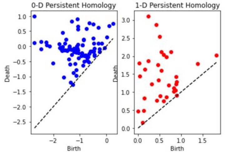
When I find the persistence diagrams using cubical homology and using the natural grayscale filtration of the image, I get two different answers depending on the package I use. By inspection, it seems that the package cripser gives the expected persistence diagram, and giotto-tda gives a persistence diagram that does not make sense to me. My questions is, why do giotto-tda and cripser give different persistent diagrams?

Here I will give a reproducible example, and point out the differences in the persistence diagrams.

You can find instructions to download cripser here, and instructions to download giotto-tda are here.

First, cripser does not come with plotting functions, so I've made one here that you may use for the example below, but feel free to ignore it:

import numpy as np
import matplotlib.pyplot as plt
import cripser
def get_2d_pd(gray_image): '''Takes a 2d numpy array and produces the persistence diagram data in a format specified at return cripser.computePH(gray_image, maxdim=1)
def display_2d_pd(pd, disp_db_locs = False): b0 = np.array([x[1] for x in pd if x[0]==0]) x0 = np.linspace(np.min(b0), np.max(b0)) d0 = np.array([x[2] for x in pd if x[0]==0]) d0[-1] = np.max(d0[:-1])*1.1 #make infinite death value 10% more than all other death values b1 = np.array([x[1] for x in pd if x[0]==1]) x1 = np.linspace(np.min(b1), np.max(b1)) d1 = np.array([x[2] for x in pd if x[0]==1]) fig, ax = plt.subplots(1,2) ax[0].plot(x0, x0, 'k--') ax[0].scatter(b0, d0, color = 'b') ax[0].set_xlabel('Birth') ax[0].set_ylabel('Death') ax[0].set_title('0-D Persistent Homology') ax[1].plot(x1, x1, 'k--') ax[1].scatter(b1, d1, color = 'r') ax[1].set_xlabel('Birth') ax[1].set_ylabel('Death') ax[1].set_title('1-D Persistent Homology') if disp_db_locs: lbl0 = np.array([ [x[3], x[4], x[6], x[7]] for x in pd if x[0]==0]) lbl0_dict = {} lbl1 = np.array([ [x[3], x[4], x[6], x[7]] for x in pd if x[0]==1]) lbl1_dict = {} for i, lbls in enumerate(lbl0): pt = (b0[i], d0[i]) if pt in lbl0_dict.keys(): lbl0_dict[pt].append(lbls) else: lbl0_dict[pt] = [lbls] for pt, lbls in lbl0_dict.items(): txt = '' for lbl in lbls: txt += '('+str(lbl[0])+', '+str(lbl[1])+'), ('+str(lbl[2])+', '+str(lbl[3])+') \n' ax[0].annotate(txt, pt) for i, lbls in enumerate(lbl1): pt = (b1[i], d1[i]) if pt in lbl1_dict.keys(): lbl1_dict[pt].append(lbls) else: lbl1_dict[pt] = [lbls] for pt, lbls in lbl1_dict.items(): txt = '' for lbl in lbls: txt += '('+str(lbl[0])+', '+str(lbl[1])+'), ('+str(lbl[2])+', '+str(lbl[3])+') \n' ax[1].annotate(txt, pt) plt.show()

Here is the main example:

# Generate a random 20 by 20 array
from numpy.random import default_rng
rng = default_rng(1)
vals = rng.standard_normal((20,20))
#Plot a grayscale of the image
from gtda.plotting import plot_heatmap
import plotly.express as px
plot_heatmap(vals)
#Get persistence diagram using giotto-tda
from gtda.homology import CubicalPersistence
cubical_persistence = CubicalPersistence(n_jobs=-1)
rand_vals = cubical_persistence.transform(vals)
cubical_persistence.plot(rand_vals)
#Get persistence diagram using cripser and helper functions defined above
cripser_pd = get_2d_pd(vals)
display_2d_pd(cripser_pd)

Result from giotto-tda

Result from cripser

Original Image

Notable differences

• First, gtda does not detect any 1D homology while cripser does. Why?
• Second, for 0D homology, gtda detects many less components than cripser.
• Finally, the components that gtda does detect do not have the same birth and death values as the components detected by cripser.

Any help on clarifying why I have gotten two seemingly inconsistent outputs would be much appreciated!

$\endgroup$ 0

1 Answer

$\begingroup$

Ok, I'm not 100% this is the solution, but it's worth giving a shot. As you can see here here, there are two ways to build a filtered cubical complex on a grid, the V-construction (pixels are 0 cells, equivalent to 4-adjacency) and the T-construction (pixels are top-dimensional cells, equivalent to 8-adjacency). Cripser apparently computes the V-construction by default, whereas Giotto, if it indeed uses GUDHI as backend, uses the T-construction, see here.

The paper Duality in Persistent Homology of Images shows that the duality between the persistence of the V- and T-constructions requires you to dualize the height function, which in this case just means replacing "vals" with "-1*vals", and the resulting persistence won't be exactly the same, but will be equivalent up to a beautiful symmetry (taken from their paper):

In summary, there are two, dual conventions for doing cubical persistence on grids, and the symmetry between them requires you to flip the height function and then flip/negate some of the bars across different homological degrees.

$\endgroup$

Your Answer

Sign up or log in

Sign up using Google Sign up using Facebook Sign up using Email and Password Submit

Post as a guest

Post Your Answer Discard

By clicking “Post Your Answer”, you agree to our terms of service, privacy policy and cookie policy