VLOOKUP won't work unless text is retyped manually even after cleaning and trimming
 Sebastian Wright
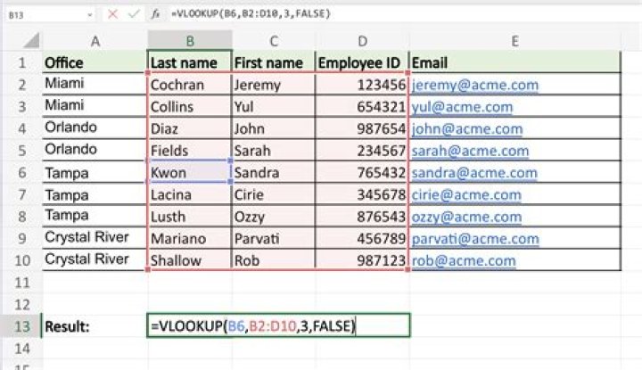
I have been having this problem with the VLOOKUP function lately. I have two arrays with mostly the same data in the first column and I'm trying to stitch them together using VLOOKUP as I've always done.
However, VLOOKUP always returns #N/A, despite the key existing in the second array, unless the data in the first array is rewritten by hand. I have cleaned and trimmed the data in both arrays to try to fix it. I have formatted the relevant columns appropriately (they're both text strings). I have cleared formats, comments and notes, hyperlinks, everything. Please please help, I'm at a loss!
Here is the function I'm using:
(VLOOKUP(A2,Sheet1!$A$2:$B$5,2,FALSE)Here is an example of the two arrays:
| Player | Value |
|---|---|
| Cade Cunningham | #N/A |
| Jordan Nwora | #N/A |
| Luka Doncic | #N/A |
| Player | Value |
|---|---|
| Jordan Nwora | 1.5 |
| Luka Doncic | 1.3 |
| Cade Cunningham | 2.1 |
1 Answer
The telling point made is unless the data in the first array is rewritten by hand: this means, to about a five sigma certainty, that there are still non-happy characters in the strings, even after trimming and cleaning.
Even without that point, this would almost certainly be the case given the steps you have taken.
I would especially direct attention to the fact that non-printing characters are often non-visible as well, except to someone looking, carefully, for precisely them.
They literally take no actual space in the line of text you see when you enter the formula editor (with F2, say). They simply do not seem to exist, visible in no way whatsoever except for one physical test. One can use other tests, formulas for instance, but physically, only the "arrow" test is effective.
For that, enter Edit mode (F2) on one such cell that is giving an error when its value is looked up. Note the cursor at the end of the text in the cell. Or click at the end to have it start there. Using the ← key, slowly, or at least carefully, move toward the start of the text. What you are looking for is a moment when the key is pressed, but the cursor doesn't move left. Oops, must've not quite pressed it. No, you pressed it, it's just that you found one of the characters giving you trouble.
At this point, and if it is as one hopes, that there is just a single such character occurring throughout the data, not several, you can move the cursor over the next character to be sure of your place, then back, then move it one more character rightward but with the Shift key pressed, note that it seems not to move again, then one more character noting it gets highlighted too, then back left so it unhighlights. You should now have only the invisible character highlighted. Copy it to the Clipboard.
Exit the cell, then press Ctrl+H to bring up Find and Replace, and replace all instances of this character by pasting it into the Find what: entry line.
See if some or all of the lookups now provide good answers. If "all", then that my be all you need to do. If only "some", there are more to find in the continued error-return pieces of data.
You can select some empty cell, enter Edit Mode, and paste this character into it. Then in another cell, use the UNICODE() function (NOT the CODE() function) to get is decimal code. You can record that for use on future downloads of the data.
Using Excel's CLEAN() function especially, or finding sites recommending you also Find and Replace a short list of characters, doesn't really work well. The CLEAN() function was like a version 1.0 (or 0.7...) on the idea and has never been updated. The lists you find are like a version 2.0, or so, in that they were the characters websites started using after programs got functionality like Excel's CLEAN() function. For whatever reason, website programmers do not want you removing these characters so they keep using new ones. I won't say they are trying to screw us when we "screen scrape" but it does come to mind. More likely they are trying to stay ahead of