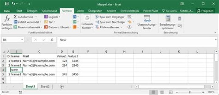
I have two Excel spreadsheets. On the first sheet is a list of people's names with other data in the rest of the columns. In the second sheet, the first column is linked to the names in the first sheet (using "='Sheet1'!B1", etc); however, the rest of the columns in the second sheet are different types of data from the first sheet. If I want to move a name on the first sheet, this would automatically move the same name on the second sheet, but it won't bring the rest of the data with it. Is there a way to do this so that data follow the name?

7

3 Answers

I doubt there is an "canonical answer" because the "problem" is not canonical for Excel. In other words: Excel, which is a spreadsheet application, is not made to solve such problems.

Your assumption "the first column is linked to the names in the first sheet (using "='Sheet1'!B1", etc); " is wrong. The formula ='Sheet1'!B1 does not link to names. The formula result is what value is in 'Sheet1'!B1. If that value changes, the formula result also changes. That is exactly what you observe and call a "problem".

Linked tables are typical for a relational database system. There one table may have foreign keys to link to another table. See Foreign key. But Excel is not a relational database system.

There is Power Query to create a data query from Excel Tables which also is able to have foreign key relations between tables. But this is not really straightforward. So let's have a very simple example:

First create a workbook having two sheets having a data table each.

Example

Data of Sheet1:

Name Mail Value1
Name1 [email protected] 123
Name2 [email protected] 234
Name3 [email protected] 234

Name of the Table is Data1

Data of Sheet2:

Name Value2
Name2 2345
Name1 1234

Name of the Table is Data2

Now create a Power Query from Table Data1. See Import from an Excel Table

• Select a cell in Table Data1 (is on Sheet1).
• Select Data > Get & Transform Data > From Table/Range.
• Excel opens the Power Query Editor with your data displayed in a preview pane.
• To return the transformed data to Excel, select Home > Close & Load.

You get an additional sheet having the result of that data query. For me that sheet gets named "Data1".

Now do the same with Table Data2.

• Select a cell in Table Data2 (is on Sheet2).
• Select Data > Get & Transform Data > From Table/Range.
• Excel opens the Power Query Editor with your data displayed in a preview pane.
• To return the transformed data to Excel, select Home > Close & Load.

You get an additional sheet having the result of that data query. For me that sheet gets named "Data2".

Now select the sheet "Data1" (The sheet which holds the first query result) and edit the query. See Create, load, or edit a query in Excel (Power Query) - > Edit a query from a worksheet -> To edit a query, locate one previously loaded from the Power Query Editor, select a cell in the data, and then select Query > Edit.

Now merge queries from Data1 with the one from Data2. See Merge queries (Power Query) -> Perform aMerge operation.

• Select Home > Merge Queries.
• The Merge dialog box appears.
• Select the primary table from the first drop-down list, and then select a join column by selecting the column header. This is column "Name" in our case.
• Select the related table from the next drop-down list, and then select a matching column by selecting the column header. This is table "Data2" and column "Name" in our case.
• Select OK.

The result should be an new column "Data2" added to the query "Data1".

Now select the handle at right side of column name "Data2" and mark only "Value2" selected. The coulmn name should change to "Data2.Value2"

To return the transformed data to Excel, select Home > Close & Load.

Result should be the data table on sheet "Data1" cahnged to show the Value2 of Data2 too.

From now on all changes in Table "Data1" on Sheet1 and in Table "Data2" on Sheet2 will be put together on query result on Sheet "Data1" when you refresh that query.

Disclaimer: This answer is for the linked example in Automatically move an entire row of reference cell when one cell is moved or manipulated.

In Google Sheets, you can use the =QUERY() function to automatically move an entire row when one cell on another sheet changes.

Here is an example of how you can use the =QUERY() function to move an entire row from one sheet to another when a specific cell changes:

In the sheet where you want to move the row, create a new column and name it "Status."
In the sheet where the cell that will trigger the move is located, create a new column and name it "Move."
In the "Move" column, use an IF() statement to check if the cell you want to trigger the move is true or false. For example: =IF(A1=TRUE,"Move","Stay")
In the sheet where you want to move the row, use the =QUERY() function to select the rows where "Move" is "Move" and "Status" is not "Moved". For example: =QUERY(Sheet1!A1:Z,"select * where Move = 'Move' and Status != 'Moved'")
In the sheet where the cell that will trigger the move is located, use the =IF() statement to change the value of the "Status" column to "Moved" when "Move" is "Move". For example: =IF(Move="Move","Moved",Status)
Use a script to automatically run the query and update the status every time the cell that triggers the move is changed.

Please note that this is an example and you will need to modify the formulas and sheet names to match your specific use case.

hope this helps

1

As the question is not really clear about this, there would be another approach if you have the following structure:

Given following data in Sheet1:

ID Name Mail Value1 Value2
1 Name1 [email protected] 123 1234
2 Name2 [email protected] 234 2345
3 Name3 [email protected] 345 3456

Now Sheet2 shall only pull different data from Sheet1 dependent on Name. Then Sheet2 could have following formulas filled downwards from row 2:

A2: =Sheet1!B2

B2:C4: =VLOOKUP($A2,Sheet1!$B$1:$E$998,MATCH(Sheet2!B$1,Sheet1!$B$1:$AAA$1,0),FALSE)

Now you can change data in Sheet1 and Sheet2 will always show the correct data for name because of the formulas.

Your Answer

Sign up or log in

Sign up using Google Sign up using Facebook Sign up using Email and Password Submit

Post as a guest

Post Your Answer Discard

By clicking “Post Your Answer”, you agree to our terms of service and acknowledge that you have read and understand our privacy policy and code of conduct.