How do you derive the backward differentiation formula of 3rd order using interpolating polynomials?
 Matthew Martinez
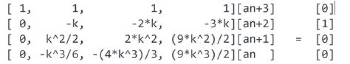
It was my exam question, and I could not answer it. How do you drive the backward differentiation formula of 3rd order (BDF3) using interpolating polynomials? I only knew how to derive it using the undetermined coefficients method.
BDF3 : $x_{n+1} = \frac{18}{11}x_{n} - \frac{9}{11}x_{n-1} + \frac{2}{11}x_{n-2} + \frac{6}{11}hx_{n+1}$
$\endgroup$ 41 Answer
$\begingroup$I'll start with the way I think you know and then discuss the method which uses explicit interpolation scheme. I'll note that the differences are mostly semantic and lead to the same answer, but it never hurts to know how to approach a problem from multiple angles.
Let's say we want to find the value of $x_{n+1}$ that balances the differential equation
$$ \frac{\mathrm{d}x}{\mathrm{d}t}=f(t,x) $$
at $t=t_{n+1}$ given we know $x_{n-2}$, $x_{n-1}$, and $x_{n}$ at times $t_{n-2} = t_{n+1}- 3 \Delta{t}$, $t_{n-1} = t_{n+1}- 2 \Delta{t}$, and $t_{n} = t_{n+1}- \Delta{t}$, respectively, and we have no closed form for $x(t)$.
One way to approach the problem is to express the derivative of $x(t)$ on the left-hand side of the ODE as a linear combination of the three values we know in addition to the value we're searching for:
$$ \frac{\mathrm{d}x}{\mathrm{d}t}\bigg\rvert_{t_{n+1}} = \omega_{n+1} x_{n+1} + \omega_{n} x_{n} + \omega_{n-1} x_{n-1} + \omega_{n-2} x_{n-2}. $$
In order to determine the coefficients of the combination, we can replace the known values with suitable Taylor Expansions about $t_{n+1}$:
$$ \begin{align} x_{n} &= x_{n+1} + (-1\Delta{t}) \frac{\mathrm{d}x}{\mathrm{d}t}\bigg\rvert_{t_{n+1}} + \frac{(-1\Delta{t})^2}{2!} \frac{\mathrm{d}^2 x}{\mathrm{d}t^2}\bigg\rvert_{t_{n+1}} + \frac{(-1\Delta{t})^3}{3!} \frac{\mathrm{d}^3 x}{\mathrm{d}t^3}\bigg\rvert_{t_{n+1}} + \mathcal{O}(\Delta{t}^{4}) \\ x_{n-1} &= x_{n+1} + (-2\Delta{t}) \frac{\mathrm{d}x}{\mathrm{d}t}\bigg\rvert_{t_{n+1}} + \frac{(-2\Delta{t})^2}{2!} \frac{\mathrm{d}^2 x}{\mathrm{d}t^2}\bigg\rvert_{t_{n+1}} + \frac{(-2\Delta{t})^3}{3!} \frac{\mathrm{d}^3 x}{\mathrm{d}t^3}\bigg\rvert_{t_{n+1}} + \mathcal{O}(\Delta{t}^{4}) \\ x_{n-2} &= x_{n+1} + (-3\Delta{t}) \frac{\mathrm{d}x}{\mathrm{d}t}\bigg\rvert_{t_{n+1}} + \frac{(-3\Delta{t})^2}{2!} \frac{\mathrm{d}^2 x}{\mathrm{d}t^2}\bigg\rvert_{t_{n+1}} + \frac{(-3\Delta{t})^3}{3!} \frac{\mathrm{d}^3 x}{\mathrm{d}t^3}\bigg\rvert_{t_{n+1}} + \mathcal{O}(\Delta{t}^{4}) \end{align}. $$
As will be shown, the expansions were carried out to third-order to create a solvable (square) system. For other numerical methods, the number of needed Taylor Expansions (in this problem, three) and needed order (in this problem, again, three) may increase or decrease as needed to effect a solution.
As an aside, by examining the pattern from the expansions above, it is easy to see that for this constant $\Delta{t}$ problem, the general form of the Taylor Expansions is
$$ x_{n-k} = x_{n+1} + \sum_{m=1}^p \frac{[-(k+1) \Delta{t}]^m}{m!} \frac{\mathrm{d}^m x}{\mathrm{d}t^m}\bigg\rvert_{t_{n+1}} + \mathcal{O}(\Delta{t}^{p+1}), $$
where for this problem, $k \in \{0,1,2\}$ (mapping to $x_n$, $x_{n-1}$, and $x_{n-2}$) and $p = 3$ for the third order expansions. This generalization is limited to only constant $\Delta{t}$ methods but can be used in computer algebra systems to create generic code to calculating various other order methods for these systems. Aside over.
Substituting these three Taylor Expansion equalities into the linear combination gives
$$ \begin{align} \frac{\mathrm{d}x}{\mathrm{d}t}\bigg\rvert_{t_{n+1}} = &\left[\omega_{n+1} + \omega_{n} + \omega_{n-1} + \omega_{n-2}\right] x_{n+1} \\ &\left[(-1\Delta{t}) \omega_{n} + (-2\Delta{t}) \omega_{n-1} + (-3\Delta{t}) \omega_{n-2}\right] \frac{\mathrm{d}x}{\mathrm{d}t}\bigg\rvert_{t_{n+1}} \\ &\left[\frac{(-1\Delta{t})^2}{2!} \omega_{n} + \frac{(-2\Delta{t})^2}{2!} \omega_{n-1} + \frac{(-3\Delta{t})^2}{2!} \omega_{n-2}\right] \frac{\mathrm{d}^2x}{\mathrm{d}t^2}\bigg\rvert_{t_{ n+1}} \\ &\left[\frac{(-1\Delta{t})^3}{3!} \omega_{n} + \frac{(-2\Delta{t})^3}{3!} \omega_{n-1} + \frac{(-3\Delta{t})^3}{3!} \omega_{n-2}\right] \frac{\mathrm{d}^3x}{\mathrm{d}t^3}\bigg\rvert_{t_{ n+1}} &+ \mathcal{O}(\Delta{t}^{4}) \end{align}. $$
In the above expression, there is a first-order derivative at $n+1$ on the left-hand side and several different orders of derivatives on the right-hand side. In order to give the best approximation, we seek weights that zero the coefficients of the zeroth-, second-, and third-order derivatives and gives a coefficient of one for the first-order derivative:$$ \begin{align} \omega_{n+1} + \omega_{n} + \omega_{n-1} + \omega_{n-2} &= 0 \\[1em] (-1\Delta{t}) \omega_{n} + (-2\Delta{t}) \omega_{n-1} + (-3\Delta{t}) \omega_{n-2} &= 1 \\[1em] \frac{(-1\Delta{t})^2}{2!} \omega_{n} + \frac{(-2\Delta{t})^2}{2!} \omega_{n-1} + \frac{(-3\Delta{t})^2}{2!} \omega_{n-2} &= 0 \\[1em] \frac{(-1\Delta{t})^3}{3!} \omega_{n} + \frac{(-2\Delta{t})^3}{3!} \omega_{n-1} + \frac{(-3\Delta{t})^3}{3!} \omega_{n-2} &= 0 \end{align}. $$
This can be expressed as a square, linear system:
$$ \begin{bmatrix} 1& 1&1&1\\ 0&-1\Delta{t} & -2\Delta{t} & -3\Delta{t}\\ 0& \frac{1}{2!}(-1\Delta{t})^2 &\frac{1}{2!}(-2\Delta{t})^2&\frac{1}{2!}(-3\Delta{t})^2\\ 0& \frac{1}{3!}(-1\Delta{t})^3 & \frac{1}{3!}(-2\Delta{t})^3 & \frac{1}{3!}(-3\Delta{t})^3 \end{bmatrix} \begin{bmatrix} \omega_{n+1}\\\omega_{n}\\\omega_{n-1}\\\omega_{n-2} \end{bmatrix} = \begin{bmatrix} 0\\1\\0\\0 \end{bmatrix}. $$
The solution of this system leads to the linear combination:
$$ \frac{\mathrm{d}x}{\mathrm{d}t}\bigg\rvert_{t_{n+1}} = \frac{1}{\Delta{t}} \left(\frac{11}{6} x_{n+1} - 3 x_{n} + \frac{3}{2} x_{n-1} - \frac{1}{3} x_{n-2}\right) + \mathcal{O}(\Delta{t}^4) $$
where the equality becomes approximate when the higher-order terms are omitted.
Another approach to take is to use the information we have and the conditions we want to form a local cubic approximation to $x(t)$. Consider the following polynomial
$$ \hat{x}(t) = c_0 + c_1 (t - t_{n+1}) + c_2 (t - t_{n+1})^2 + c_3 (t - t_{n+1})^3. $$
If $\hat{x}(t)$ exactly matches the three points we know in addition to the value we're searching for at their associated times, it may be a good approximation of $x(t)$ close to $t_{n+1}$. And if $\hat{x}(t)$ is a good approximation, it's derivative may approximately balance the ODE at $t_{n+1}$:
$$ \frac{\mathrm{d}x}{\mathrm{d}t}\bigg\rvert_{t_{n+1}} \approx \frac{\mathrm{d}\hat{x}}{\mathrm{d}t}\bigg\rvert_{t_{n+1}} = c_1 $$
Note that because we're clever and centered the polynomial on $t_{n+1}$, only the $c_1$ coefficient remains after evaluation of the derivative at that time.
Through the four requirements on the polynomial to match our four points-of-interest, we can form the linear system
$$ \begin{bmatrix} 1 & 0 & 0 & 0 \\ 1 & -1 \Delta{t} & (-1 \Delta{t})^2 & (-1 \Delta{t})^3\\ 1 & -2 \Delta{t} & (-2 \Delta{t})^2 & (-2 \Delta{t})^3\\ 1 & -3 \Delta{t} & (-3 \Delta{t})^2 & (-3 \Delta{t})^3 \end{bmatrix} \begin{bmatrix} c_0 \\ c_1 \\ c_2 \\ c_3 \end{bmatrix} = \begin{bmatrix} x_{n+1} \\ x_n \\ x_{n-1} \\ x_{n-2} \end{bmatrix} $$
and obtain the value of the needed coefficient
$$ c_1 = \frac{1}{\Delta{t}} \left(\frac{11}{6} x_{n+1} - 3 x_{n} + \frac{3}{2} x_{n-1} - \frac{1}{3} x_{n-2}\right) $$
This answer agrees with the approximation from the Taylor Expansion method after neglecting higher-order terms.
Both are valid approximations and merely differ in how the problem is approached:
- Directly approximate the derivative of an unknown function with values we know and a cubic Taylor approximation about the point-of-interest.
- Directly approximate the unknown function with values we know using a cubic polynomial and evaluate its derivative at the point-of-interest.
Would the answer be the same if we used a different basis for the interpolation such as Lagrange versus the above Monomial? It shouldn't since all one-dimensional interpolating polynomials of degree $n$ are unique given $n+1$ interpolation points. But let's check.
Consider the following polynomial
$$ \hat{x}(t) = \sum_{j=-2}^{1}\,\prod_{\substack{-2\le m \le 1\\ m \neq j}} \frac{t - t_{n+m}}{t_{n+j} - t_{n+m}} \,x_{n+j} $$
It would be rather verbose and tedious to look at all of the terms, so let's focus on the $j = 1$ term of the polynomial:
$$ \frac{(t-t_{n})(t-t_{n-1})(t-t_{n-2})}{(t_{n+1}-t_n)(t_{n+1}-t_{n-1})(t_{n+1}-t_{n-2})} x_{n+1} $$
We can compress the denominator to $6 \Delta{t}^3$ since the interval $\Delta{t}$ is fixed between all points, and we note that the derivative of the product in the numerator is a summation of lower degree products:
$$ \frac{\mathrm{d}}{\mathrm{d}t}\left[(t-t_{n})(t-t_{n-1})(t-t_{n-2})\right] = (t-t_{n})(t-t_{n-1}) + (t-t_{n})(t-t_{n-2}) + (t-t_{n-1})(t-t_{n-2}) $$
which is equal to $11 \Delta{t}^2$ when evaluated at $t_{n+1}$. So the coefficient for the $x_{n+1}$ coefficient is $\tfrac{11}{6 \Delta{t}}$, which is the same as the two above results.
Performing the process for each other value of $j$ will also generate the same terms.
$\endgroup$ 14