difference between the statistical power calculated by statsmodels.stats.power.TTestIndPower.solve_power and the area under the PDF curve
 Sebastian Wright
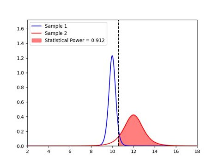
I am trying to evaluate the statistical power of a test.
Let's suppose I have two indipendent samples with these properties:
| sample | number of observations | mean | standard deviation |
|---|---|---|---|
| 1 | 10 | 10 | 1 |
| 2 | 5 | 12 | 2 |
and let's considering a significance level of 0.05.
I can use statsmodels.stats.power.TTestIndPower.solve_power to compute the power of this test, but I have to compute the effect size and the pooled standard deviation (square root of pooled variance).
import numpy as np
from statsmodels.stats.power import TTestIndPower
n1 = 10 # number of observations of sample 1
n2 = 5 # number of observations of sample 2
mi1 = 10 # mean of sample 1
mi2 = 12 # mean of sample 2
sigma1 = 1 # standard deviation of sample 1
sigma2 = 2 # standard deviation of sample 2
alpha = 0.05 # significance level
s_pooled = np.sqrt(((n1 - 1)*sigma1**2 + (n2 - 1)*sigma2**2)/(n1 + n2 - 2))
effect_size = (mi1 - mi2)/s_pooled
ratio = n2/n1
power = TTestIndPower().solve_power(effect_size = effect_size, power = None, nobs1 = n1, ratio = ratio, alpha = alpha, alternative = 'smaller')
Which gives me a power of: 0.801.
Now I want to draw a plot of samples probability density functions and related statistical power.By definition, statistical power is the area under the probability density function of the alternative hypothesis (sample 2) starting from the significance level of null hypothesis (consider this document as a reference).
So I can make a check and compute this area with numpy.trapz:
import numpy as np
import matplotlib.pyplot as plt
from scipy import stats
n1 = 10 # number of observations of sample 1
n2 = 5 # number of observations of sample 2
mi1 = 10 # mean of sample 1
mi2 = 12 # mean of sample 2
sigma1 = 1 # standard deviation of sample 1
sigma2 = 2 # standard deviation of sample 2
alpha = 0.05 # significance level
fig, ax = plt.subplots()
s1 = sigma1/np.sqrt(n1)
s2 = sigma2/np.sqrt(n2)
xmin = min(mi1 - 3*sigma1, mi2 - 3*sigma2)
xmax = max(mi1 + 3*sigma1, mi2 + 3*sigma2)
axis_lim = max(np.abs(mi1 - xmax), np.abs(mi1 - xmin))
N = 1000
x = np.linspace(mi1 - axis_lim, mi1 + axis_lim, N)
pdf1 = stats.t(loc = mi1, scale = s1, df = n1).pdf(x)
ax.plot(x, pdf1, color = 'blue', label = 'Sample 1')
pdf2 = stats.t(loc = mi2, scale = s2, df = n2).pdf(x)
ax.plot(x, pdf2, color = 'red', label = 'Sample 2')
limit = mi1 + s1*stats.t.ppf(1 - alpha, df = n1)
filt = x > limit
area_power = np.trapz(pdf2[filt], x[filt])
ax.fill_between(x = x[x > limit], y1 = pdf2[x > limit], color = 'red', alpha = 0.5, label = f'Statistical Power = {area_power:.3f}')
ax.axvline(x = limit, linestyle = '--', color = 'k')
ax.set_xlim(x[0], x[-1])
ax.set_ylim(0, 1.4*max(np.max(pdf1), np.max(pdf2)))
ax.legend(frameon = True)
plt.show()
I get:
Starting from the same values, statsmodels.stats.power.TTestIndPower.solve_power computes a power of 0.801 while the computed area under the curve is 0.912.
Where is the mistake? Did I make a mistake in calculating the power or drawing the graphs or both?